Image Data Augmentation using Albumentations

This article explains the importance of data augmentation in deep learning and computer vision, and issues around development models to create a robust and stable model to perform the task. This article also introduces a new format from the way I explain things in order to make readers understand and grasp the idea that I wrote.

What is Data Augmentation?

Data augmentation is a technique used in deep learning for most of unstructured data such as images, text, and audio, to artificially increase the size and diversity of a training dataset. The aim of data augmentation is to train the model to more variations of the data during training, which can supposedly improve its ability to generalize and perform better on unseen data during evaluation or inference.

When should you use data augmentation?

Data augmentation is particularly useful in computer vision tasks when one or more of the following conditions are met:

1. Limited training data, When the available training data is relatively small or limited, data augmentation can help increase the dataset size and expose the model to more variations, improving its ability to generalize. Limited training data here is like 1K to 10K images with multi-classes.

2. High variance: If the real-world scenarios in which the model will be deployed involve a high degree of variance or diversity (e.g., varying lighting conditions, object orientations, camera angles), data augmentation can help the model learn to handle these variations.

3. Invariance requirements: In tasks where the model needs to be invariant to certain transformations, such as recognizing objects regardless of their position, scale, or orientation, data augmentation can help the model learn these invariances.

4. Overfitting prevention: Data augmentation can act as a regularization technique, introducing variations and noise to the training data, which can help prevent overfitting and improve the model's generalization capabilities.

5. Class imbalance: When the dataset has an imbalance in the number of samples across different classes, data augmentation can be applied to oversample the underrepresented classes, improving the model's ability to learn from minority classes.

6. Domain-specific requirements: In certain domains, such as medical imaging or industrial inspection, data augmentation can be tailored to introduce variations that are relevant and important for the specific task at hand.

It's important to note that while data augmentation can be beneficial in many computer vision tasks, it should be applied judiciously and with an understanding of the problem domain. Inappropriate or excessive augmentation techniques may introduce unrealistic variations that can harm the model's performance or lead to overfitting to the augmented data.

Additionally, data augmentation should be coupled with other best practices, such as using a separate validation set to monitor the model's performance and tuning hyperparameters appropriately. It's also crucial to evaluate the model's performance on a representative test set that resembles real-world scenarios to ensure that the augmentation techniques have indeed improved the model's generalization capabilities.

How to use data augmentation in computer vision tasks?

One could use opencv or any other python imaging library, but I found Albumentation useful for speed up data augmentation process.
Albumentations is a Python package designed for rapid and versatile image augmentation techniques. It delivers a diverse range of optimized image transformation operations aimed at boosting performance. Despite its efficiency, Albumentations offers a straightforward yet robust interface for applying image augmentations across various computer vision applications, such as object classification, segmentation, and object detection tasks.

How to use data augmentation using Albumentations?

pip install -U albumentations

How does Albumentation performance compare to other libraries?

The benchmark evaluated the performance of various data augmentation libraries by measuring their throughput on the first 2000 images from the ImageNet validation dataset using an AMD Ryzen Threadripper 3970X CPU. The results showcase the number of images processed per second on a single core, where a higher value indicates superior performance. Notably, Albumentations outperformed other prominent libraries like TorchVision, Kornia, Augly, and Imgaug in terms of processing speed for this benchmark, demonstrating its efficiency in applying augmentation operations to image data.

How does Albumentations perform in action?

There are two ways, when you implement data augmentation. Either you generate first and put all of them to jpg files, or compute on the fly in data loader. In this article I show you how to product an image and then later you can save to jpg file.

Load modules

import cv2
import albumentations as A
import matplotlib.pyplot as plt

Check version, I am using 1.4.6

A.__version__

Load image and convert BGR to RGB. OpenCV by default load the image to BGR format.

im_arr = cv2.imread('000000000025.jpg')
im_arr = cv2.cvtColor(im_arr, cv2.COLOR_BGR2RGB)

Display image

plt.imshow(im_arr)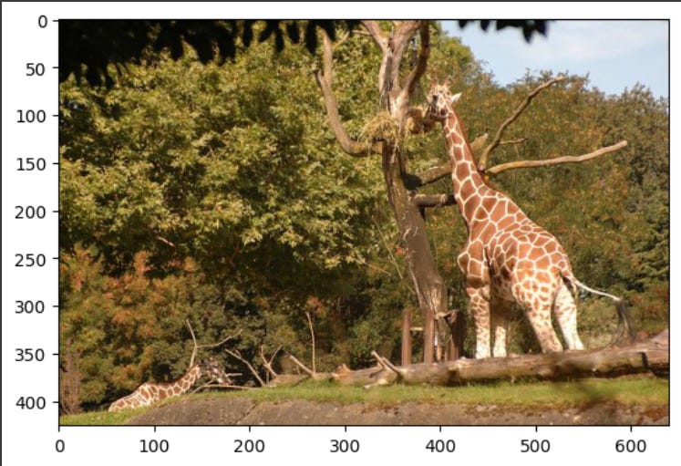

Then, we can try to manipulate images.

# Random Brightness Contrast
RBC = A.RandomBrightnessContrast(brightness_limit=1, contrast_limit=1, p=1.0)
im_arr_rbc = RBC(image=im_arr)['image']

# Advanced Blur
AB = A.AdvancedBlur(blur_limit=81, 
                    sigma_x_limit=(1.0, 10.0), sigma_y_limit=(0.2, 1.0),
                    rotate_limit=(-90, 90),
                    beta_limit=(0.5, 8.0),
                    noise_limit=(0.75, 1.25),
                    p=1)
im_arr_ab = AB(image=im_arr)['image']

# Blur
B = A.Blur(blur_limit=21, p=1.0)
im_arr_b = B(image=im_arr)['image']

# Flip
F = A.Flip(p=1.0)
im_arr_f = F(image=im_arr, d=0)['image']

# Horizontal Flip
HF = A.HorizontalFlip(p=1.0)
im_arr_hf = HF(image=im_arr)['image']

# Hue Saturation Value (HSV), Hue = 100, others = 0
HSV_H = A.HueSaturationValue(hue_shift_limit=100, sat_shift_limit=0, val_shift_limit=0, 
                           p=1.0)

im_arr_hsv_h = HSV_H(image=im_arr)['image']

# HSV, Saturation = 100, others 100
HSV_S = A.HueSaturationValue(hue_shift_limit=0, sat_shift_limit=100, val_shift_limit=0, 
                           p=1.0)

im_arr_hsv_s = HSV_S(image=im_arr)['image']

Then, we can plot all the images

fig, axes = plt.subplots(2, 4, figsize=(20, 6))
axes[0, 0].imshow(im_arr)
axes[0, 0].axis('off')
axes[0, 0].set_title('Original')
axes[0, 1].imshow(im_arr_rbc)
axes[0, 1].axis('off')
axes[0, 1].set_title('Random Brightness Contrast')
axes[0, 2].imshow(im_arr_ab)
axes[0, 2].axis('off')
axes[0, 2].set_title('Advanced Blur')
axes[0, 3].imshow(im_arr_b)
axes[0, 3].axis('off')
axes[0, 3].set_title('Blur')

axes[1, 0].imshow(im_arr_f)
axes[1, 0].axis('off')
axes[1, 0].set_title('Flip')

axes[1, 1].imshow(im_arr_hf)
axes[1, 1].axis('off')
axes[1, 1].set_title('')

axes[1, 2].imshow(im_arr_hsv_h)
axes[1, 2].axis('off')
axes[1, 2].set_title('HSV Hue')

axes[1, 3].imshow(im_arr_hsv_s)
axes[1, 3].axis('off')
axes[1, 3].set_title('HSV Saturation')

Closing

That’s it for this article. If you like and currently learning computer vision, consider to follow and subscribe this newsletter.